How to count and sum values by fill and font color
Contents
How to count and sum values by fill and font color
Begin Function by Color
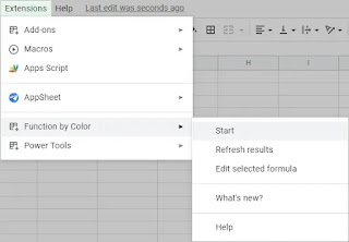
Go to Extensions > Color Functions >Start in the Google Sheets menu to access the utility:
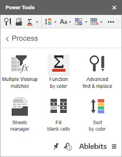
Tip. You will also find the add-on in Power Tools, which is a collection of all Ablebits add-ons for spreadsheets:
- Open Extensions > Power Tools > Start in the Google Sheets menu:
- Then either click on the tool icon and pick the Function by Color option:
How to count and sum values by fill and font color
You will see the add-on pane with a few settings to adjust:
- Define the range of cells where you want to calculate colored cells. Tip: Select a range of cells before running the tool, and they will be picked up for processing. But if you run the add-on with a single active cell in the sheet, that cell will be taken as a place for the result.
To change the range, just enter it manually or click the Select range icon. The latter will open a special window, allowing you to pick the necessary cells:
Tip: Use the Auto Select button for the tool to identify your table (a used range until the first blank row and column) automatically. - Decide on the background and font colors that you want to calculate.
- Click the Color Picker button, and you will get a pop-up window inviting you to select a pattern cell from your sheet:
- Once the pattern cell is chosen, the font color and background color icons in the add-on will feature the corresponding hues. The checkboxes next to these icons let you decide if you want to calculate cells that share only the font color, the background color, or both hues.Tip. You can change these text and fill colors or set them from the beginning. Just click the corresponding icon and either pick the required shade from the palette or enter its hex code in a special field:
- Click the Color Picker button, and you will get a pop-up window inviting you to select a pattern cell from your sheet:
- Single out the function you want to use for calculations from the Use function drop-down list. You can choose between the following functions: SUM, COUNT (to count numeric values only), COUNTA (to count both numeric and textual values), COUNTBLANK, AVERAGE, AVERAGEA, MIN, MAX, PRODUCT, MODE, STDEV, VAR, MEDIAN. Tip. If your task is to count cells with a particular color, it is best to choose COUNTA, as it is the only function that works with text values.
- Select or enter the destination cell for the Function by Color formula in the Paste Results To field. You can select the top-left cell for the results, and the add-on will automatically adjust the range based on the next option.
- Use the calculator in the list to do one of the following:
- Insert one formula for the entire range:
- calculate each column individually:
- count colored cells in each row in the range, respectively:Tip. This way, if you want to check how many green cells there are in each row, you won’t have to copy the formula manually.
- Insert one formula for the entire range:
- Check the final checkbox to have the add-on fill results with your pattern colors (the hues used for calculations).
- If you don’t frequently use the last two options (calculate in and fill results with your pattern colors), click the upward-pointing arrow icon to hide them.You can make them visible again at any time by clicking the arrow once more.
Hit the Insert function to calculate all cells in the desired range based on the selected colors.
Note: To our regret, Google Sheets takes some time to calculate custom formulas. If you have a large table, please wait a few seconds before the value of the built-in formula changes from “0” to a correct one.


.webp)

